GROUP MEMBERS

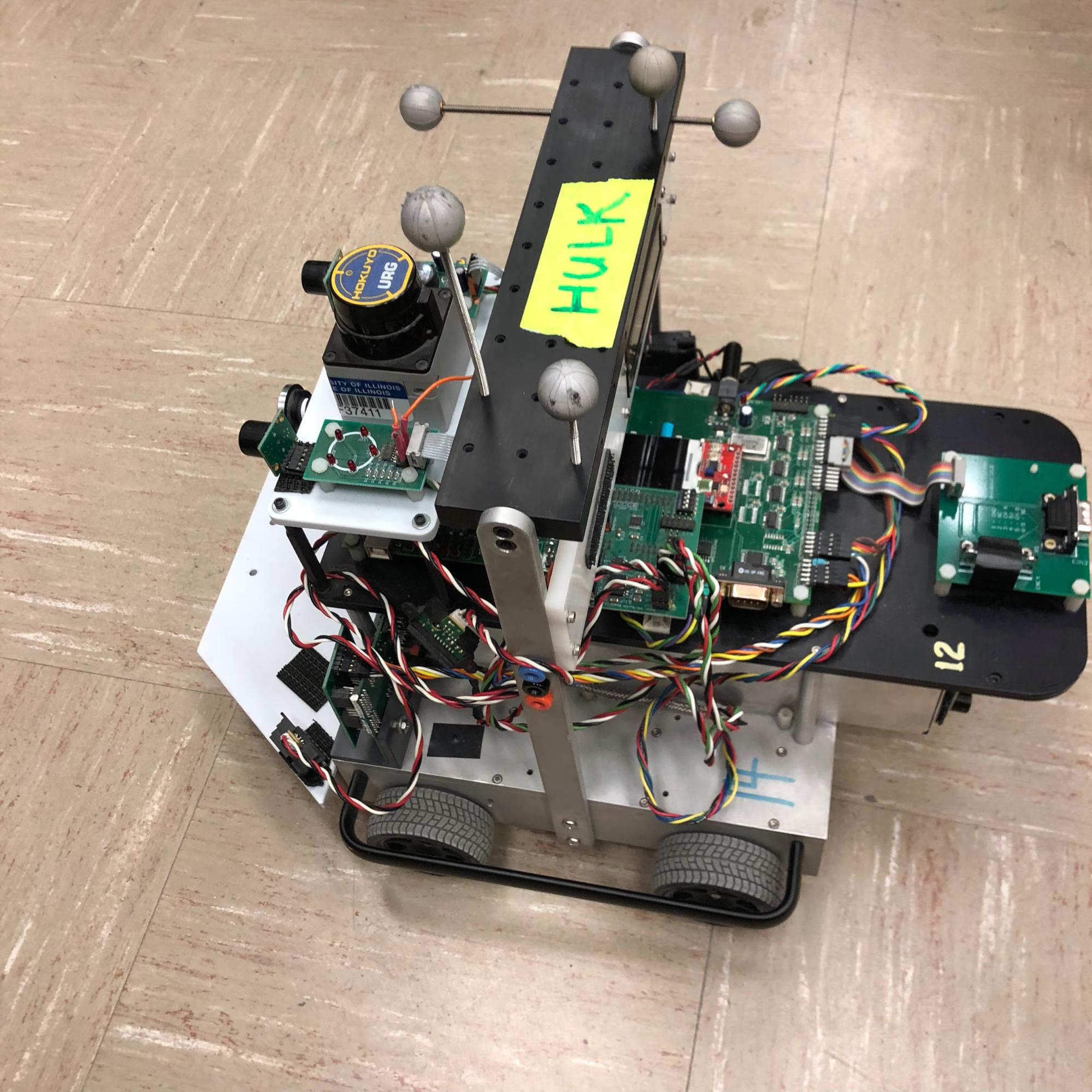
   Hulk

IDENTIFYING THE TARGET POSITION

Every time it loops through the camera screen, only the biggest colored area will be regarded as the target and has its information sent from the color vision to the ‘RobotControl’ function. After receiving the information, the robot will first turn to the target and calculate its position after the projection of the target is right on the column center of the camera (we gave it a little off set for our camera is crooked). The position will be stored and sent to the ‘xy control’ as the next destination if the comparison shows that it hasn’t be found before. And after finding one target, it will ignore the camera information for a while to avoid repeatedly turning. And into the switch case loop in ’RobotControl’, the sequence of killing the weeds is: turning to the largest pink target, comparing and storing the position; turning to the largest blue target, comparing and storing the position; heading towards the pink location using ‘xy control’, and then the blue location; setting the ‘currCase = 2’, breaking out and waiting for re-astaring to the next destination in case 2. If any step in this sequence is blank, the robot will skip it and continue.

BUG ALGORITHM (BACKUP PLAN)

While path planning, if the robot detects a wall, wall following algorithm will be called. The position where the robot enters the wall following loop will also be recorded as the start position. The robot then follows the wall until it reaches a point where it’s on the straight line path from the start position to target position. It breaks out from the loop and goes back to path planning loop.

A* PATH PLANNING

However it takes a long time for the robot to go through the whole course with only the bug algorithm. In order to make the robot smarter and use less time to finish explore the course, some advanced algorithm need to be used, which is the A* search algorithm. With a good heuristic function, the A* is guarenteed to return the best path. However that is only theoretical, which considers only the total length of the path. In reality, even the paths with the same length will take different times. A path with less turns will take a shorter time than a path with more turns. Under such circumstance, we modified the heuristic function of the A* algorithm, and add a small number to the function if the current step is a turn, so that when the algorithm search the next node, it will automatically search the path with less turns. The other problem for the A* algorithm is that the algorithm requires to know the setup of the course in order to decide the best path. As a result, we add wall detecting to the program. Every time when the robot detects there is a wall near it, it go through the 288 values of the ladar. In order to avoid hit the wall, the robot will go back a little bit for enough room to make a turn. According to the absolute x and y coordinates of the obstacle detected, it can plot the wall on the course and notified the A* algorithm to re-plan a path. In order to reduce the wall that are detected mistakenly, we only consider the middle of the wall, which must be at a odd x even y coordinate or a odd y even x coordinate.

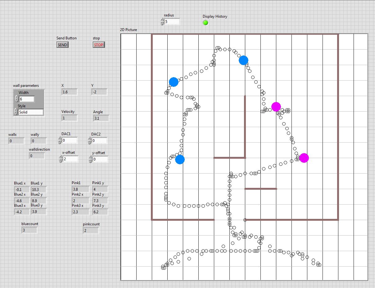
DISPLAYING ON THE LABVIEW

For the LabVIEW portion of the contest, the code that had been developed since lab 5 was used as a base point. From here, capabilities were added such that LabVIEW would draw the outline of the course, the positions of the weeds and the positions of any found obstacles during any given run. In addition, the x and y coordinates of each weed were printed to the LabVIEW front panel. These tasks were primarily accomplished by reading in floats from robot control. In addition to reading in the robot’s x, y velocity and angle data, the new floats added are a flag which determines whether a found wall is horizontal of vertical, the x and y coordinates of the wall (top most for vertical, left most for horizontal), the count of blue weeds found, pink weeds found, and their respective x and y locations (where the robot thinks they are at when it finds them). These new drawings are then sent to the next iteration of the picture so that they stick around for future iterations. The outer wall is drawn in the same part of the code as the grid, as it will always be in the same place. Manual controls were added to the front panel for tuning wall thickness as well as the size of the circles which represent the weeds.

VIDEO

https://www.youtube.com/watch?v=sjkxb46gkZ8&list=PLwp-z5nCWTcIfgAqs9FA68o0gB3oPM2O_&index=1&t=0s